Showing posts with label Tutorial. Show all posts

Tuesday, September 10, 2013

Download a Wordpress Website Creation Checklist Spreadsheet

In the past two years I’ve created eight websites for various hobbies and niches I am interested in and that I felt were underserved in the online world. I use Wordpress as my content management system because it allows you to quickly create a website with no HTML or other coding experience. The steps to setup a new website are pretty much the same so I put together a Wordpress website creation checklist to help me remember to do everything. I’ve made this checklist into an Excel template which you can download for free by clicking the link below.
 
wordpress website creation checklist
 
Two skills I encourage everyone to learn that I’ve found invaluable in my career is how to program VBA macros and how to build a simple website. In fact, in one of my most recent projects these skills were used hand-in-hand. I built the majority of the Observation Wheel database with an Excel spreadsheet and a few custom macros. Every row in my sheet contained all the information for a single observation wheel. I then had the macro export the data to Microsoft Word in the HTML format I needed for the site. I then simply copied and pasted that text into Wordpress and published it. I created pages for over eighty dfferent observation wheels almost instantly!
 
There are countless positive benefits for learning how to make a website. I’ve included a link to all the resources I use within the template and I've tried to include as many tips as I could think of. I begin with registering a domain name and take you all the way through setting up an email list. Download my Wordpress website creation checklist below and please feel free to ask me any questions you may have!
 

Wednesday, July 24, 2013

How to Filter Data in Excel

Learning how to filter data in Excel will help you analyse data faster and become better at your job. Filtering in Excel enables you to display only the data that you want to see on your spreadsheet without deleting anything. It’s a really great way to search through large amounts of information and you know I’m all about Excel tips that help improve your speed and efficiency!
add a filter in excel


There are three types of filters in Excel: list of values, by format, or criteria and you can sort your spreadsheet by order, color or text. What’s the difference between sorting and filtering? Sorting will rearrange the order of your list while filtering keeps the order but actually hides data based on your filter criteria.


To add a Filter in Excel, you can first select a single cell within your range of data but I recommend you highlight all your data (please note you cannot add filters to empty cells). Next, go to the Home tab then the Editing section. Under Sort & Filter click Filter (or use the filter shortcut Crtl+Shift+L). Once filtering is turned on you will see little arrows along your top row of data. Select one of the arrows to set your filter options. If you hover your mouse over the drop down arrow you will see a pop-up message displaying what the value the filter is currently set to (example: equals “Test”).
 
how to filter data in excel


To remove the filtering from your spreadsheet, simply click the Filter button again. If you want to reset the filter to the original values click on the Sort & Filter button and then click “Clear."


You can also turn auto-Filter on and off with a VBA macro:


Sub TurnAutoFilterOn()
'check for filter, turn on if none exists
If Not ActiveSheet.AutoFilterMode Then
ActiveSheet.Range("A1").AutoFilter
End If
End Sub


Turn off AutoFilter with VBA:


Sub TurnFilterOff()
Worksheets("Sheet1").AutoFilterMode = False
End Sub


Here’s a great video showing you exactly how to filter data in Excel:


Follow us on Google Plus for the latest updates when I will talk about dynamic filters and Kalman filters in Excel.

Thursday, June 6, 2013

Excel Pranks and Practical Jokes with VBA

I’ve shared a lot of Excel tips about how to increase your productivity at work but today I thought I would post something a little more fun – how to decrease your productivity! I’m talking about ways to use Microsoft Excel spreadsheets to play pranks, practical jokes, April Fool’s Day kind of stuff on your friends, roommates, and coworkers. The intent is not to harm anyone or hurt their professional careers – this is simply about having some plain ole fun.

A great way to wreak havoc in the workplace is to create a macro that automatically runs when an Excel workbook is opened. You can do this by writing a VBA procedure in the Open event of the workbook by using the Visual Basic Editor. Create a new Excel spreadsheet then press Alt+F11 to launch the VBA Editor. Next, right-click the ThisWorkbook object, and then click View Code.
excel pranks
 
In the Object list above the Code window, select Workbook. This will automatically create an empty procedure for the Open event like this and you can now add your evil code.

excel practical jokes
 
To make Excel automatically close itself when the workbook is opened use this:

Private Sub Workbook_Open()
     Application.DisplayAlerts = False
     Application.Quit
End Sub
 

Here’s a trick that will automatically open Microsoft Word and close Excel:

Sub Workbook_Open()
‘make sure the Microsoft Word Object Library is selected by going to tools>references
Application.Visible = False
Dim wdApp as Word.Application
Set wdApp = New Word.Application
wdApp.Visible=True
Set wdApp = Nothing
Application.DisplayAlerts = False
Application.Quit
End Sub
 

This is one of my personal favorites; have a message box pop-up asking if the user wants to download the virus they requested. Whether they press the yes or no button the next message tells them the virus has begun downloading!

Private Sub Workbook_Open()

MsgBox "The virus you requested is now ready to download, Do you want to start downloading now?", vbYesNo, "Virus Trojan-x45fju"

MsgBox "The Virus is Now Downloading. You have made the biggest mistake of your life! ByE bYe", , "Begin Virus Download"

End Sub

This function flips the workbook and will make everything on the left now appear on the right side:

ActiveSheet.DisplayRightToLeft = True

To change all cell’s color to black:

Cells.Interior.Color = RGB(0,0,0)

Instead of automatically running a macro on opening a workbook (and making it obvious you did something) you could embed a macro that only runs on certain conditions. A funny prank is a macro to change the size of the Excel window every time the user clicks on a cell:

Private Sub Workbook_SheetSelectionChange(ByVal Sh As Object, ByVal Target As Range)

Application.WindowState = xlNormal

Application.Width = Int(Rnd() * 1000) - 100

End Sub


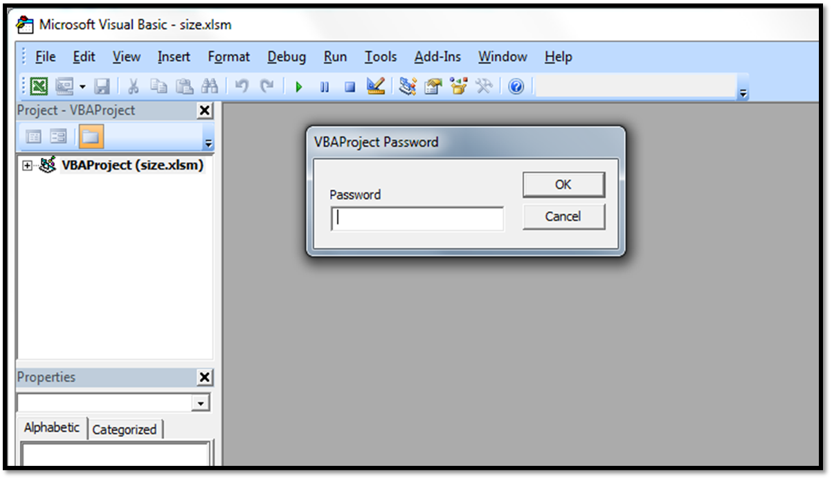
As you can imagine, the possibilities are nearly endless! Now you may think “All someone has to do is change or delete the code to fix the problem.” Well, you can protect your VBA code so only those with the password can modify it. Go to Tools>VBAProject Properties>Protection. Check the box to lock project for viewing and create a password (and remember it). Now you’re an evil genius!


Of course, if you’re not comfortable using VBA (which I recommend you get comfortable and learn it)  you can always use these old fashioned tricks:

  1. Use find and replace on a document, like replacing “you” with “you idiots”.
  2.  If your coworker has an old school mouse simply remove the ball when they're not around and then sit back and watch the fun when they try to figure out why their mouse isn't working anymore.
  3. Take a screen capture of a roommate’s desktop and save it as a jpg or bmp file. Turn on the Active Desktop, and make sure to turn off "show desktop icons". Change the wallpaper to the screen capture image you just saved and watch as they click away on their "icons" that mysteriously stopped working.

Have you ever used something like this on someone? What’s your best Excel prank?

Tuesday, March 12, 2013

How to create collapsible rows in Excel


how to group rows in excel
I was recently creating an Excel spreadsheet template for a friend and I needed to know how to create collapsible rows in Excel. I had a worksheet that listed student’s names and information. My friend wanted a +/- sign at the beginning of each row representing different groups of students that could be clicked to reveal grades for various classes. The Group function in Excel presented the perfect solution to this situation.

One method often used to collapse rows or columns in Excel is by using the Group function.

Go to the Data tab, select the rows or columns you want to group, then select the Group icon (located in the Outline are). This will result in a button being placed to the left of the row number column and allow you to instantly collapse or hide the grouped rows. To ungroup the rows simply hit the Ungroupbutton (also in the Outline area).

You can use keyboard shortcuts to improve your speed and efficiency when applying this method. First, select the Row or Column range, then;

To group:
<Shift> <Alt> <RightArrow>

To ungroup:
<Shift> <Alt> <LeftArrow>

To retain the Groups, but toggle hide/unhide the symbols:
<Ctrl> <8>
(Using the "8" that's under the function keys, *not* from the num keypad.)

Another option to group rows would be to apply Subtotals to your range.  You'll get those outlining symbols and even a subtotal row between each group. The Subtotals button is also in the Outline section of the Data tab.

I’ve created a short how to video to show you exactly how to collapse rows in Excel. Check it out below:


So that’s how you expand or collapse a group of cells in Excel. Pretty easy, huh?

-Nick

Easily Grouping Columns and Rows in Excel
Related Posts Plugin for WordPress, Blogger...