Showing posts with label Video. Show all posts

Monday, September 23, 2013

How to Combine Excel Files

There have been countless times during my day job when I’ve had to combine multiple Excel files into one. I used to do it the old fashioned way of copy and paste but after doing this tedious and time consuming task I decided to write a VBA macro to help me out. I’ve now made the template available for you to use for free. This version of the combine Excel workbooks macro allows you to choose the directory of the Excel files to copy without having to change the code in the Visual Basic Editor. The steps to use the Combine Workbooks tool are as follows:
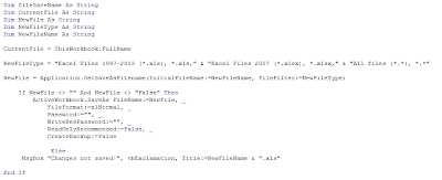
combine excel files macro
 
  1. Place the Excel workbooks you want to combine into a single folder that contains no other files
  2. Go to View>Macros
  3. Select "Combine Workbooks" then click Run
  4. Select the File where the spreadsheets you want to combine are located
  5. Save the newly created file

Instructions are provided with the spreadsheet

Please note that this code will not work on protected sheets and it will automatically skip any blank worksheets in any of the workbooks saved in the folder. See how it works for yourself by watching my short demo video below:


Download the Combine Excel Files spreadsheet that contains the VBA code to copy all the worksheets from all the workbooks in a folder into the active workbook using this link:
 

Combine Files.xlsm download

Wednesday, July 24, 2013

How to Filter Data in Excel

Learning how to filter data in Excel will help you analyse data faster and become better at your job. Filtering in Excel enables you to display only the data that you want to see on your spreadsheet without deleting anything. It’s a really great way to search through large amounts of information and you know I’m all about Excel tips that help improve your speed and efficiency!
add a filter in excel


There are three types of filters in Excel: list of values, by format, or criteria and you can sort your spreadsheet by order, color or text. What’s the difference between sorting and filtering? Sorting will rearrange the order of your list while filtering keeps the order but actually hides data based on your filter criteria.


To add a Filter in Excel, you can first select a single cell within your range of data but I recommend you highlight all your data (please note you cannot add filters to empty cells). Next, go to the Home tab then the Editing section. Under Sort & Filter click Filter (or use the filter shortcut Crtl+Shift+L). Once filtering is turned on you will see little arrows along your top row of data. Select one of the arrows to set your filter options. If you hover your mouse over the drop down arrow you will see a pop-up message displaying what the value the filter is currently set to (example: equals “Test”).
 
how to filter data in excel


To remove the filtering from your spreadsheet, simply click the Filter button again. If you want to reset the filter to the original values click on the Sort & Filter button and then click “Clear."


You can also turn auto-Filter on and off with a VBA macro:


Sub TurnAutoFilterOn()
'check for filter, turn on if none exists
If Not ActiveSheet.AutoFilterMode Then
ActiveSheet.Range("A1").AutoFilter
End If
End Sub


Turn off AutoFilter with VBA:


Sub TurnFilterOff()
Worksheets("Sheet1").AutoFilterMode = False
End Sub


Here’s a great video showing you exactly how to filter data in Excel:


Follow us on Google Plus for the latest updates when I will talk about dynamic filters and Kalman filters in Excel.

Tuesday, March 12, 2013

How to create collapsible rows in Excel


how to group rows in excel
I was recently creating an Excel spreadsheet template for a friend and I needed to know how to create collapsible rows in Excel. I had a worksheet that listed student’s names and information. My friend wanted a +/- sign at the beginning of each row representing different groups of students that could be clicked to reveal grades for various classes. The Group function in Excel presented the perfect solution to this situation.

One method often used to collapse rows or columns in Excel is by using the Group function.

Go to the Data tab, select the rows or columns you want to group, then select the Group icon (located in the Outline are). This will result in a button being placed to the left of the row number column and allow you to instantly collapse or hide the grouped rows. To ungroup the rows simply hit the Ungroupbutton (also in the Outline area).

You can use keyboard shortcuts to improve your speed and efficiency when applying this method. First, select the Row or Column range, then;

To group:
<Shift> <Alt> <RightArrow>

To ungroup:
<Shift> <Alt> <LeftArrow>

To retain the Groups, but toggle hide/unhide the symbols:
<Ctrl> <8>
(Using the "8" that's under the function keys, *not* from the num keypad.)

Another option to group rows would be to apply Subtotals to your range.  You'll get those outlining symbols and even a subtotal row between each group. The Subtotals button is also in the Outline section of the Data tab.

I’ve created a short how to video to show you exactly how to collapse rows in Excel. Check it out below:


So that’s how you expand or collapse a group of cells in Excel. Pretty easy, huh?

-Nick

Easily Grouping Columns and Rows in Excel
Related Posts Plugin for WordPress, Blogger...